Caking SXRD diffraction pattern images using DAWN
Caking diffraction pattern images using DAWN on the iCSF
iCSF
You will first need to contact IT services to get setup with an iCSF account. The iCSF (interactive Computational Shared Facility) gives us access to the University’s high performance computing environment. This allows us to store and analyse our large Synchrotron X-ray Diffraction (SXRD) datasets as a group.
What is caking?
Before we can analyse the diffraction pattern rings for changes in phase fraction, micromechanical response and texture, we need to cake the data. Caking converts our 2-dimensional image into slices (of particular azimuthal angles) to produce a number of intensity profiles versus 2-theta angle (or pixel position). We can then investigate how the intensity peak profile of particular lattice plane peaks change in particular directions over time. We can also run a full azimuthal integration, which sums up the intensities around the whole image, to produce a single intensity profile versus 2-theta angle. This can then be used to calculate the phase fraction, for instance.
Opening DAWN on the iCSF
To run the caking and azimuthal integration we have setup the program DAWN on the iCSF. DAWN is a data analysis and processing program commonly used for processing synchrotron data.
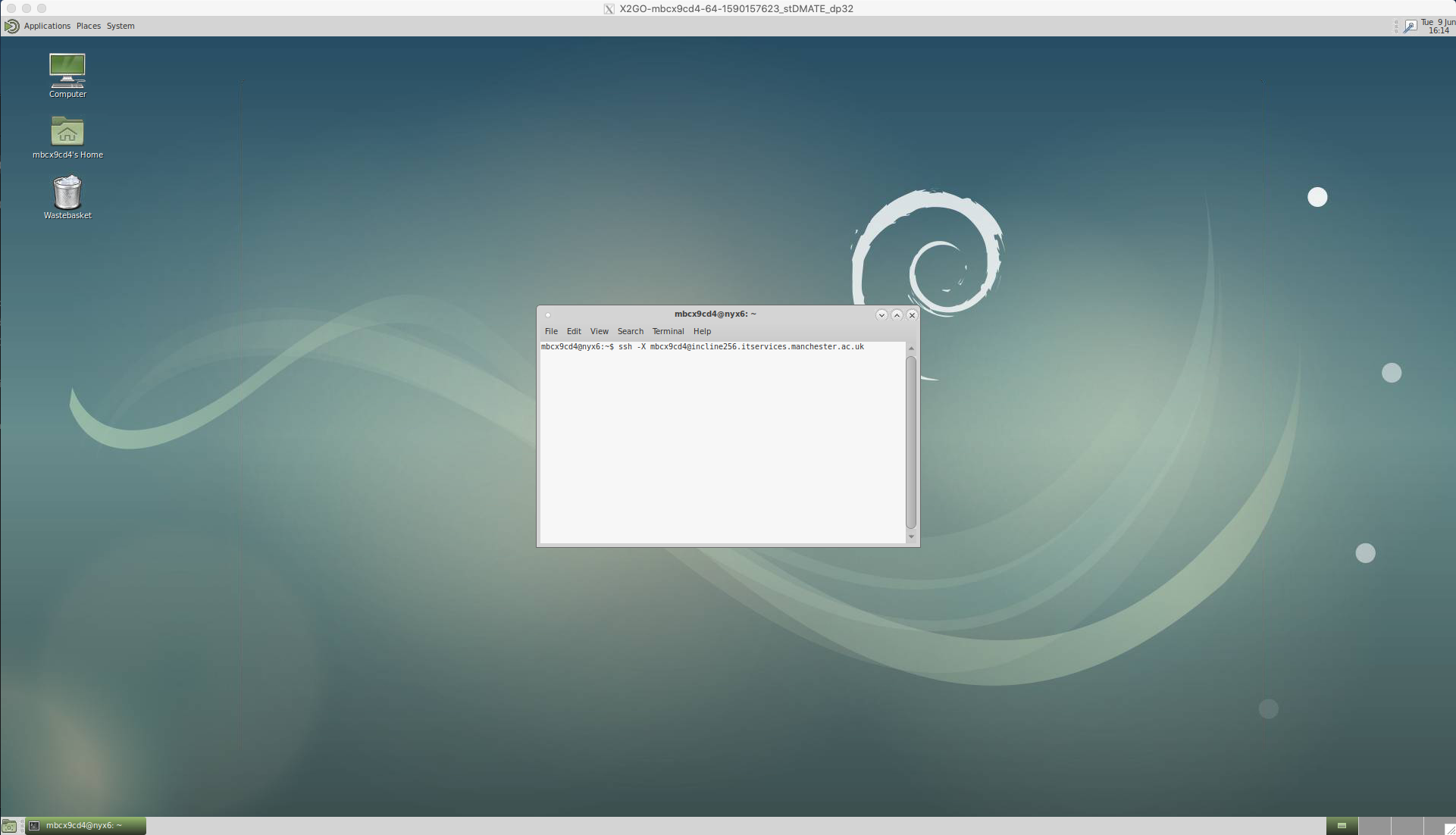
Log onto the iCSF by opening the terminal and using the secure shell (ssh) protocol;
ssh -X mbcx9cd4@incline256.itservices.manchester.ac.uk
You will then be prompted to enter your password.
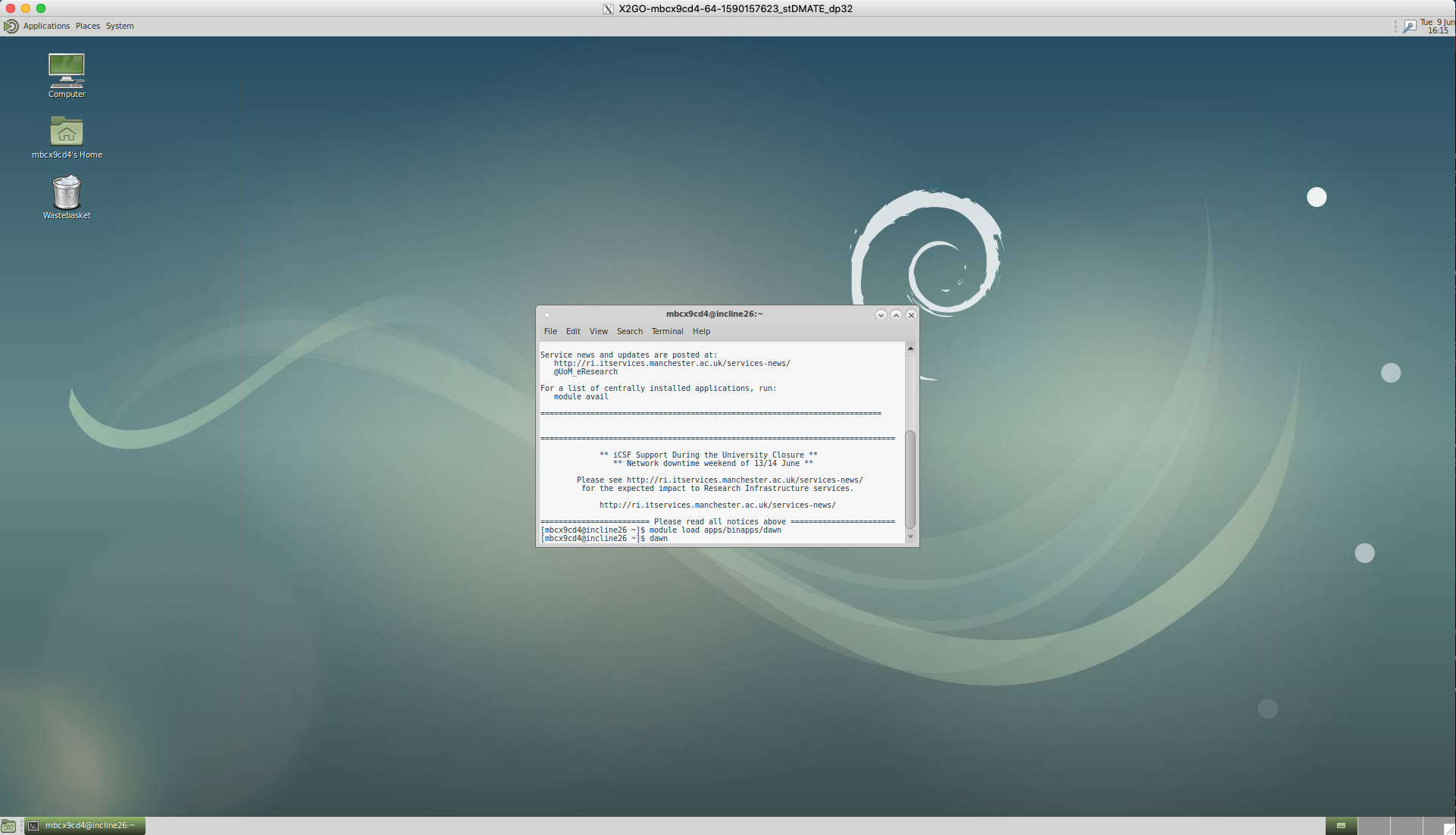
Load the DAWN module using the following commands in the terminal;
module load apps/binapps/dawn
dawn
Caking in DAWN
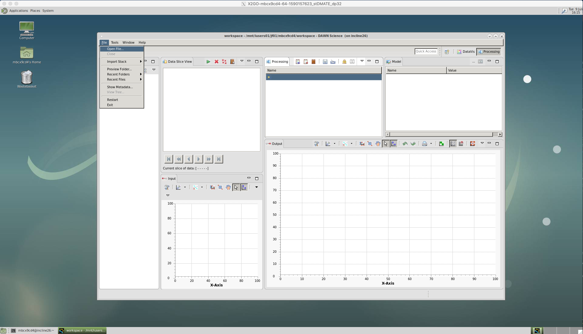
This will then open the DAWN workspace. Note, we should have the ‘processing’ window selected in the top right.
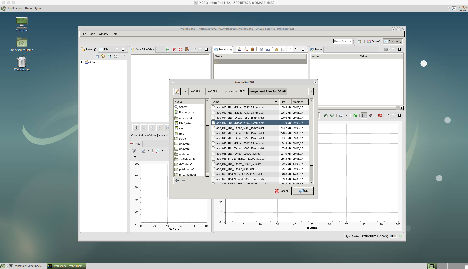
Then, clike on the ‘File’ and ‘Open File…’ tabs.
.nxs
For slower acquisition data (< 1 Hz) we have .nxs file which will have the metadata stored with the images and this can be selected.
.dat
However, for fast acquisition data (> 10 Hz) we have a .dat file which contains the metadata for each diffraction pattern image - because the image frame rate was too fast to store any additional data. This .dat file should has a couple of lines of code at the top, which instructs DAWN to load the metadata with each image and contains a file path to the rawdata i.e. the .tiff diffraction pattern images. Note, ../ means the parent directory.
&SRS
&End
path load temperature position
00001 0.002761 0.157104 0.095435
00002 0.002632 0.157179 0.095299
…
Select this .dat file and click ‘Ok’
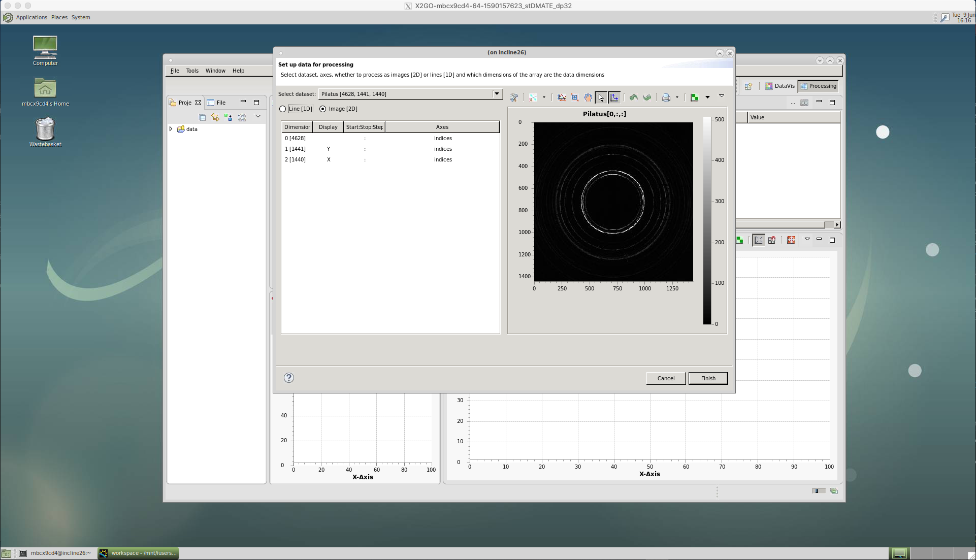
A window should appear with ‘Pilatus[x:y:z]’ showing as the ‘Select dataset’ and an image of the first diffraction pattern. The x number refers to the sequence of images that have been loaded, the y and z refer to the size of the image in pixels.
Click ‘Finish’ and the data will be loaded into the ‘Data Slice View’.
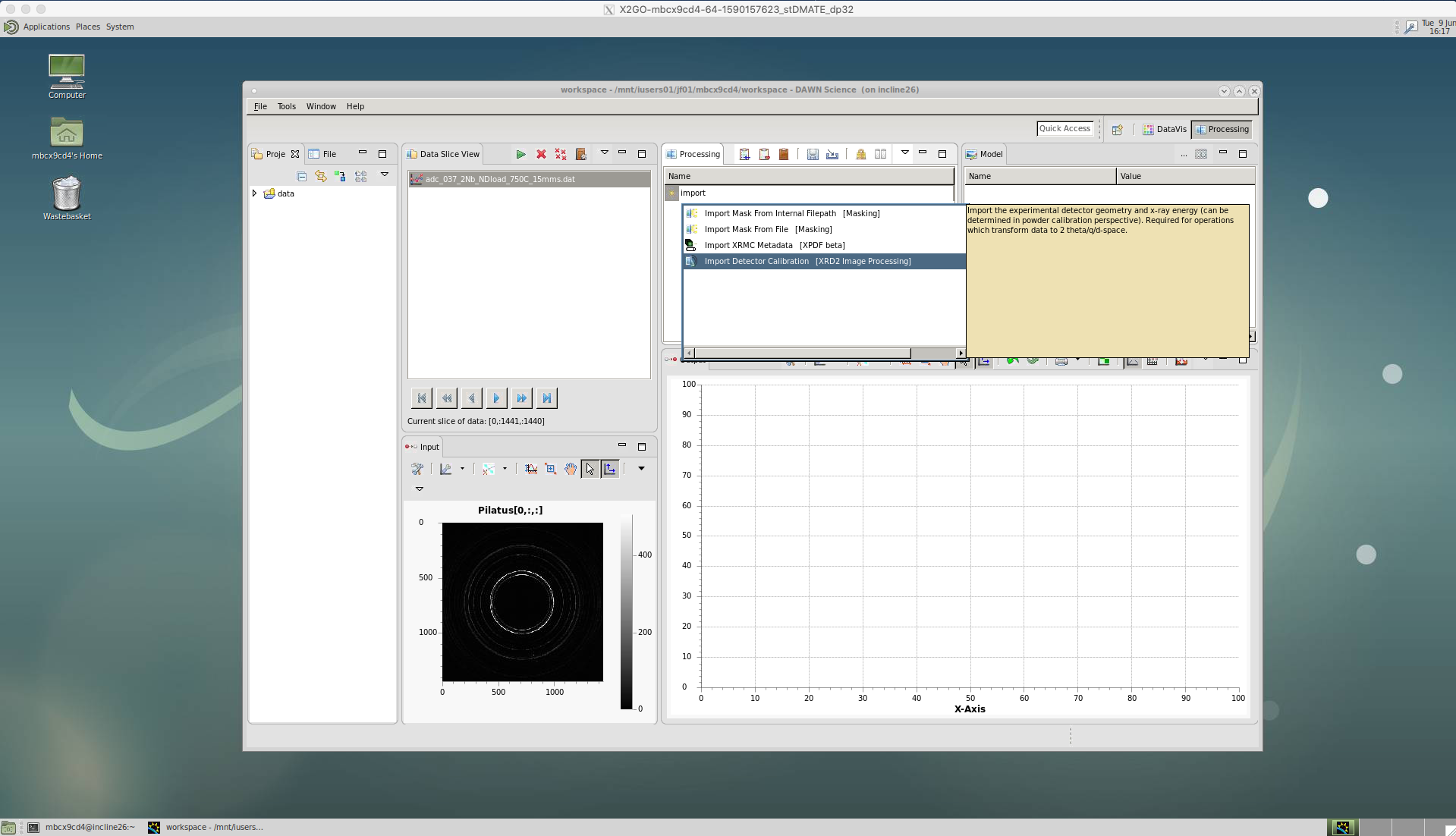
Now a particular dataset is loaded, we can setup a ‘Processing’ pipeline that will act on each image in sequence.
‘Import Detector Calibration’
Our first action is to calibrate the data. As of yet, we do not know the beam centre, the sample-detector distance, etc. and since our detector is not completely flat there will be some distortion of the diffraction pattern rings. We account for this by callibrating using an image of a known standard, typically LaB6. The calibration is done in DAWN and produces a .nxs calibration file for a particular beam/detector setup. If this calibration has not already been done, instructions are included at the end of this page.
Click on ‘Import Detector Calibration’.
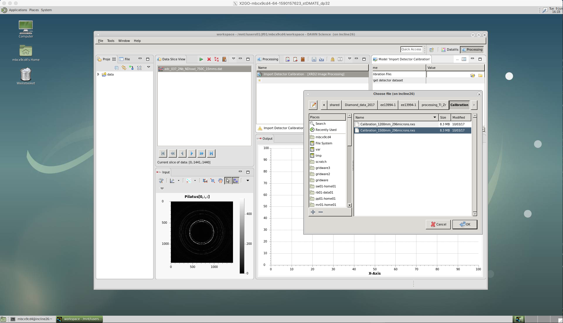
A window will appear to select the correct .nxs calibration file.
‘Threshold Mask’
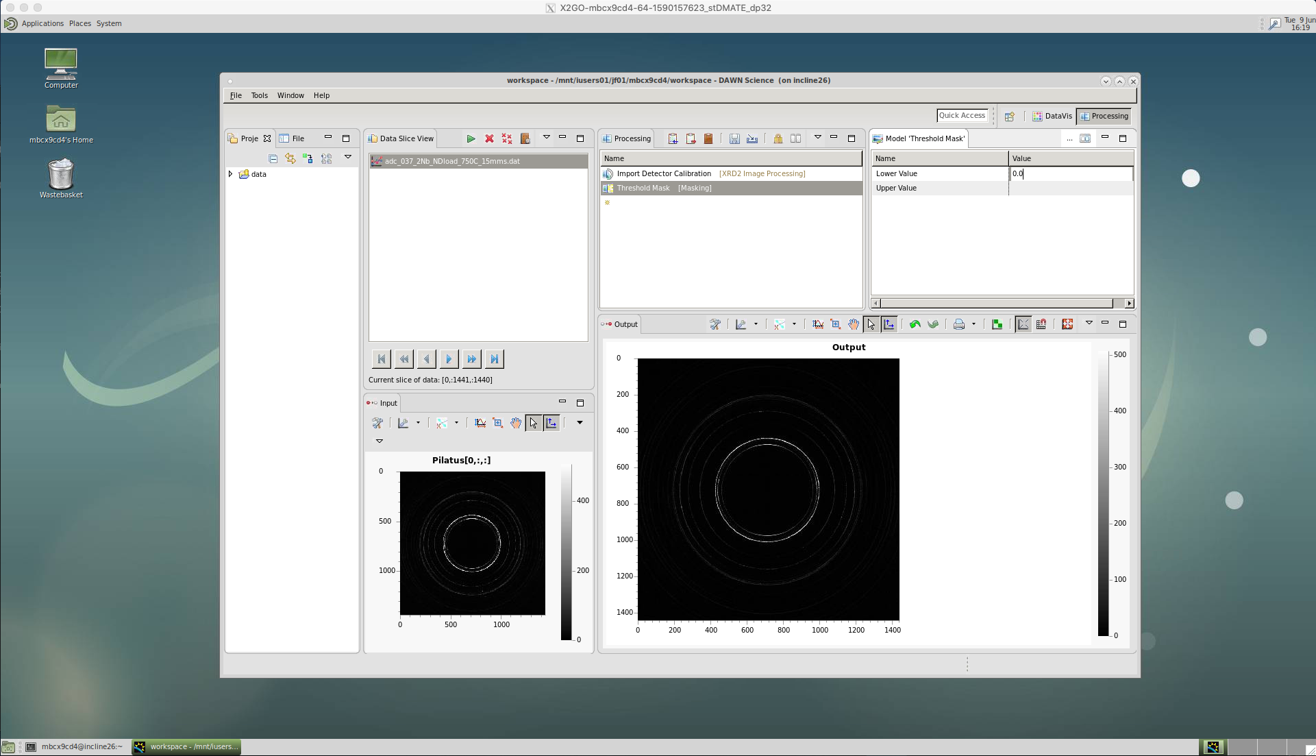
We then apply a threshold using the ‘Threshold Mask’. This is used to exclude any particularly high or low intensity counts that could occur due to dead or malfunctioning pixels on the detector. Not excluding these could affect any peak analysis of our data at a later stage.
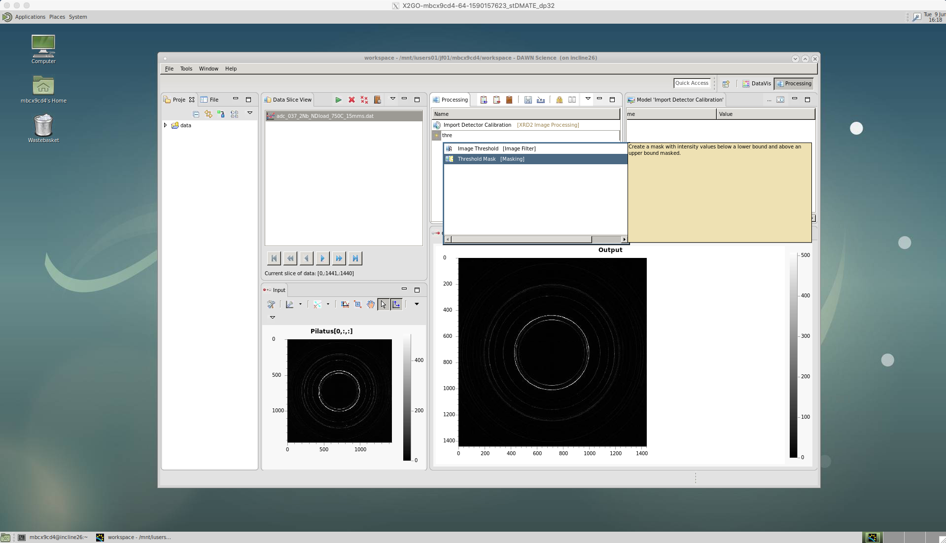
A lower value of 0.0 is chosen for Diamond’s Pixium detector. But, these values may be different for other beamlines, as well as the newer detectors at Diamond.
‘Cake Remapping’
We then apply the caking by selecting the ‘Cake Remapping’ tool.
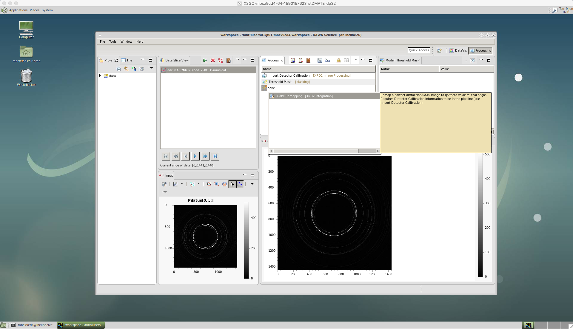
There are a number of options for ‘Cake Remapping’.
An ‘Azimuthal range’ needs to be defined, for the start and end azimuthal angles i.e. [start,end]. Zero degrees is defined as the horizontal, east direction. Here, I have selected [2.5,-357.5] since I want cakes of 5 degrees, with the first cake centred on the horizontal, east direction. Or, I could have selected [5,-355] for cakes of 10 degrees, centred on the horizontal.
The ‘Number of azimuthal bins’ should match the azimuthal range you have chosen. Here, I have selected 72, since I have 5 degree cakes covering the entire azimuthal range. Or, I could have selected 36 for 10 degree cakes. Generally, 5 degrees caking is best, since it provides a higher resolution for the subsequent analysis, particularly for texture calculation. But, if your diffraction pattern rings are spotty it helps to increase the cake width and sum over larger azimuthal angle.
‘Pixel splitting’ should be ticked. This shares the intensity between bins, which avoids step changes to the peaks and can improve single peak fitting.
The ‘X axis’ is selected as ‘Angle(degrees)’ in this case. So the intensity data will be plotted for each two-theta angle increment.
Also, make sure the ‘Zeros instead of NaNs’ is ticked. If this isn’t ticked it will cause problems loading data in Python or other software.
‘Export to Text File’
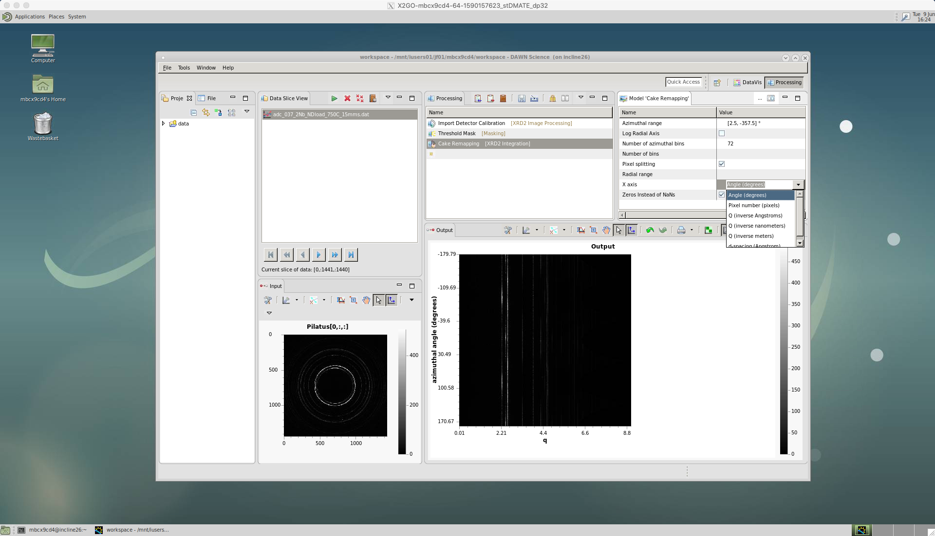
To save the caked intensity data we choose the ‘Export to Text File’ tool.
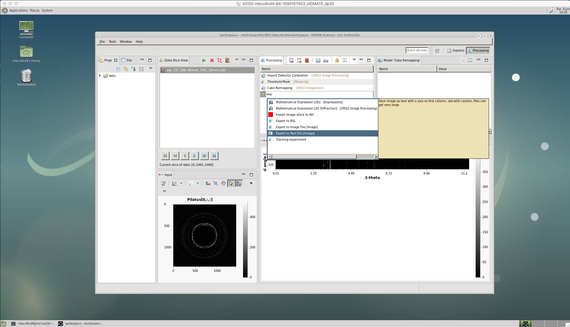
There are a number of options for ‘Export to Text File’.
You can choose any ‘File Extension’. Here, we choose ‘dat’. Note, we do not have include a dot in the file extension, as this would result in ..dat file being created. In the section below, there is an explantion of the different data types we will need to create to fully analyse our data.
Tick the ‘In separate folder’ box. This groups the data into one folder, which is useful when re-using the same pipeline to run through many different datasets.
Leave ‘Pad with zeros’ as five, which should give a high enough number count.
Then, select the ‘Output Directory’, where the data will be saved.

The processing pipeline will then run and iterate through the sequence of images, outputting the caked data files.
It is possible to view these files, which are saved to our shared research space, on your laptop. To do this, open a terminal and navigate to the Desktop. Create a new directory called ‘iCSF-Home’, or called something similar. Then, use a secure shell protocol to connect to the iCSF.
cd Desktop mkdir iCSF-Home sshfs -o follow_symlinks mbcx9cd4@incline.itservices.manchester.ac.uk: iCSF-Home
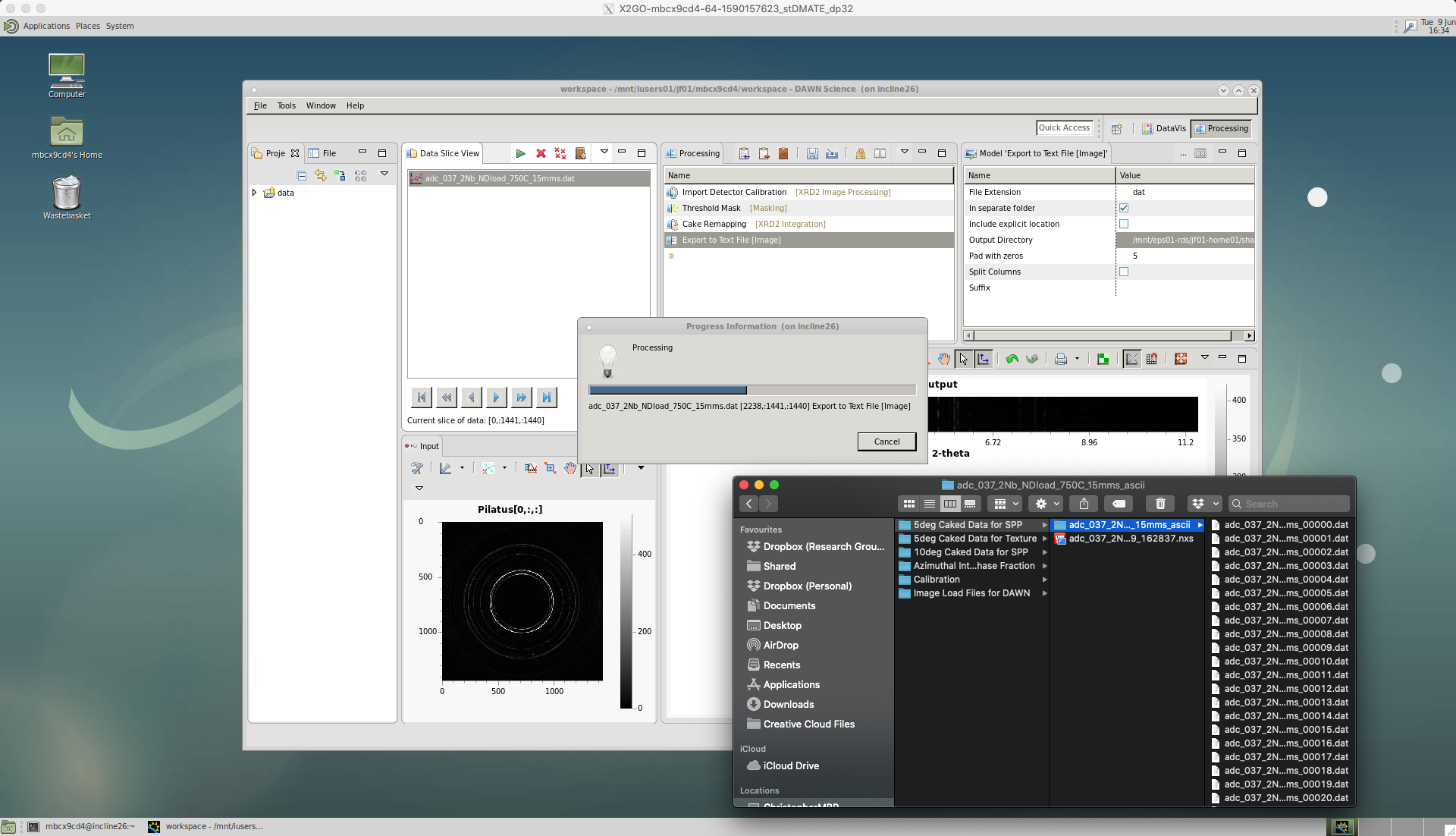
Different file formats
Single Peak Profile (SPP) with xrdfit
The above example shows the settings for saving cakes for single peak profile (SPP) analysis, which can then be loaded into xrdfit. xrdfit is a Python package for fitting and analysing the diffraction peaks, to discern the micromechanical behaviour of the material.
The key points for saving the cakes for SPP analysis in DAWN is that the ‘X axis’ is selected as ‘Angle(degrees)’ and the data is saved in ‘dat’ format.
Texture with MAUD
SXRD data can also be used to analyse changes in texture, using the MAUD software package. A Jupyter Notebook showing how to setup MAUD in batch mode is available on our shared LightForm GitHub group - MAUD-batch-analysis
The key points for saving the cakes for texture analysis in DAWN is that the ‘X axis’ is selected as ‘Pixel number (pixels)’ and the data is saved in ‘dat’ format.
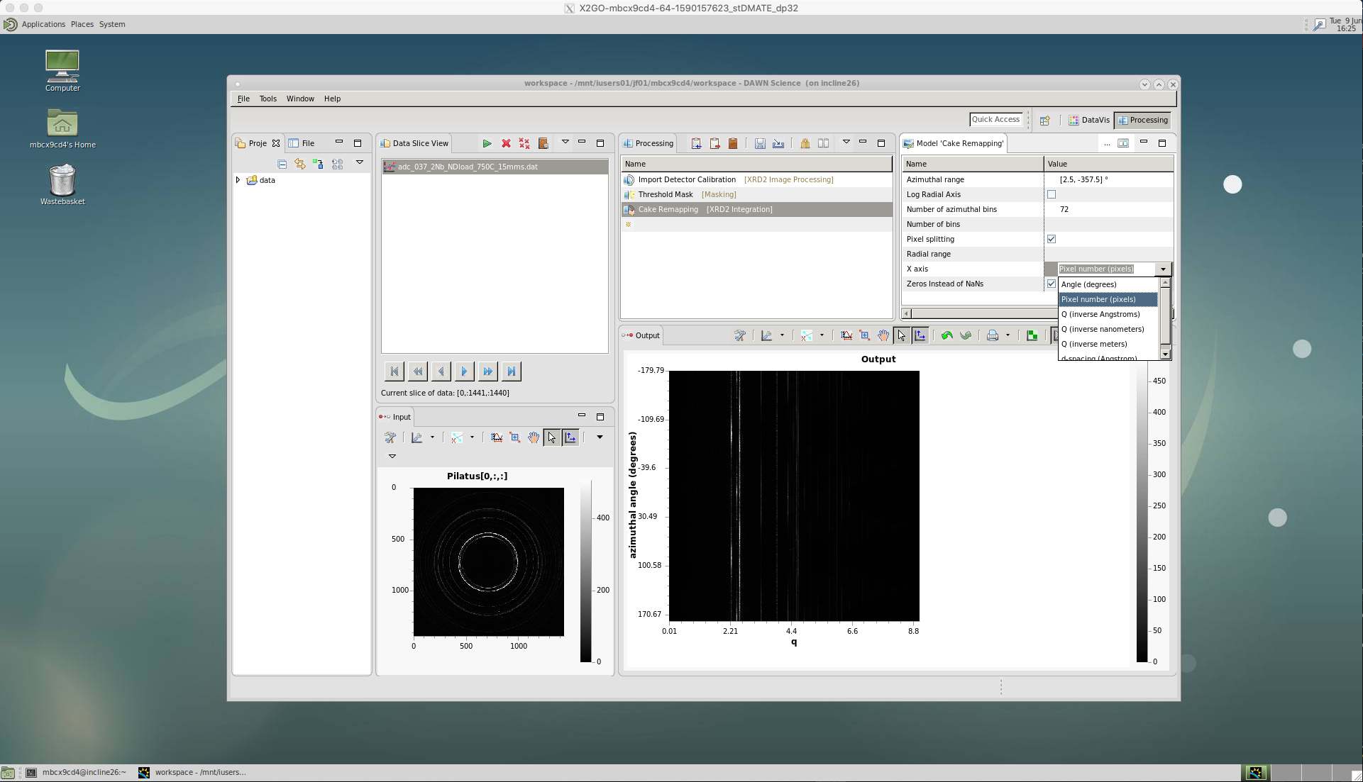
Azimuthal integration for TOPAS
DAWN can also be used to provide a full azimuthal integration, which sums up the intensities around the whole image, to produce a single intensity profile versus 2-theta angle. This can then be used to give an accurate estimation of the overall phase fraction of the material, using the program TOPAS. A Jupyter Notebook showing how to setup TOPAS batch mode is available on our shared LightForm GitHub group - TOPAS-batch-analysis
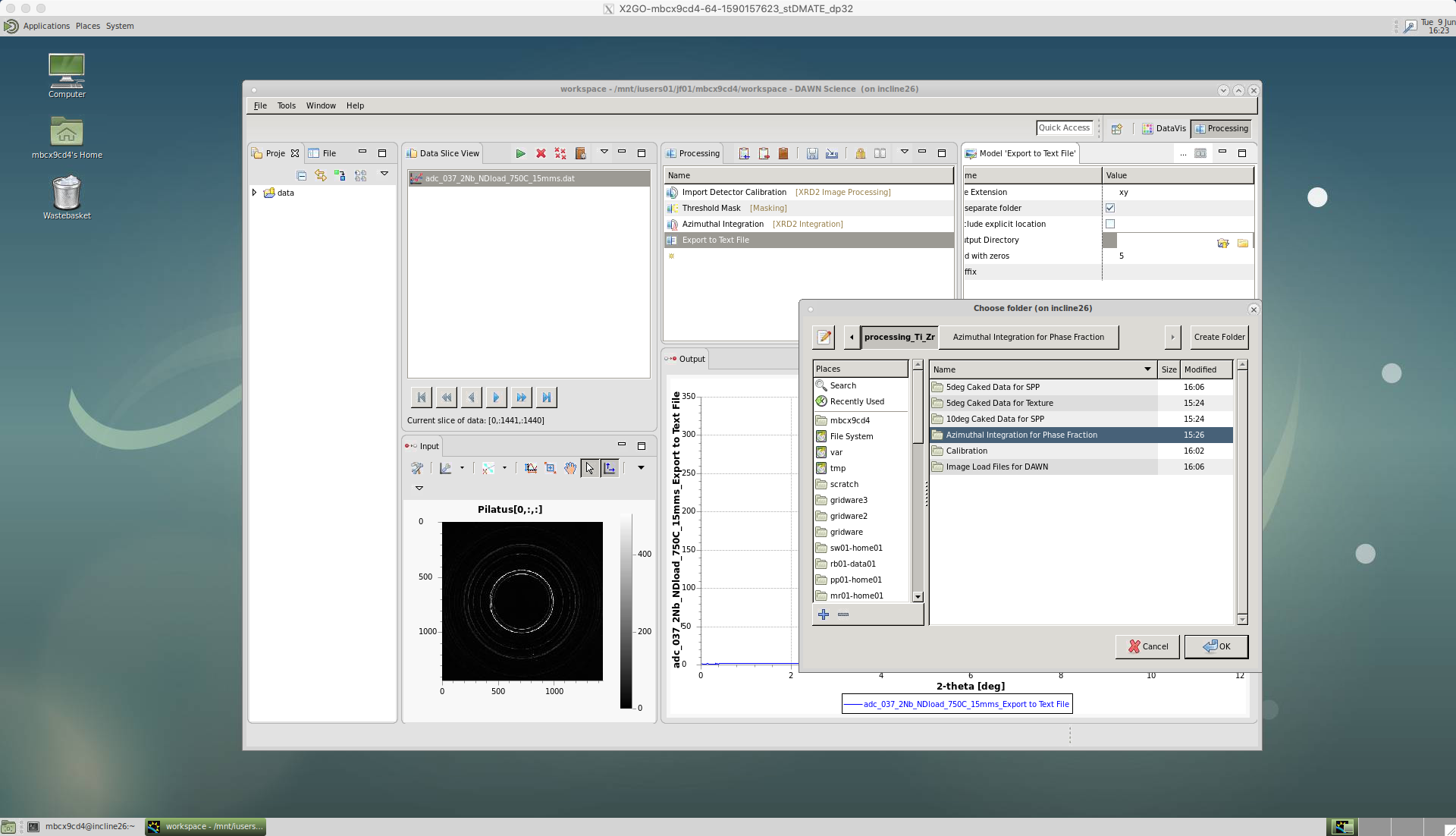
Instead of cake remapping, we now select the ‘Azimuthal Integration’ tool.
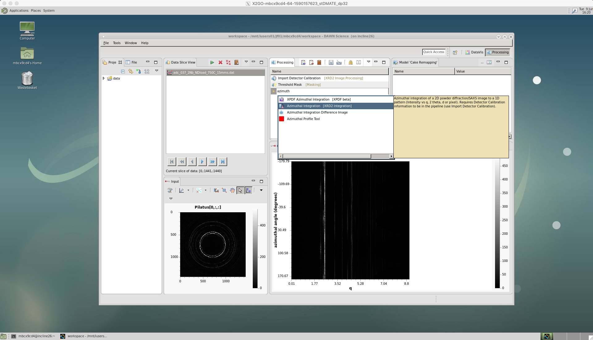
The ‘Azimuthal range’ can be left blank for a full 360 degree integration. If an area of the detector is to be avoided then a range is defined as [start,end].
‘Pixel splitting’ should be ticked. This shares the intensity between bins, which avoids step changes to the peaks and can improve single peak fitting.
The ‘X axis’ is selected as ‘Angle(degrees)’, so the intensity data will be plotted for each two-theta angle increment.
Also, make sure the ‘Zeros instead of NaNs’ is ticked. If this isn’t ticked it will cause problems in TOPAS.
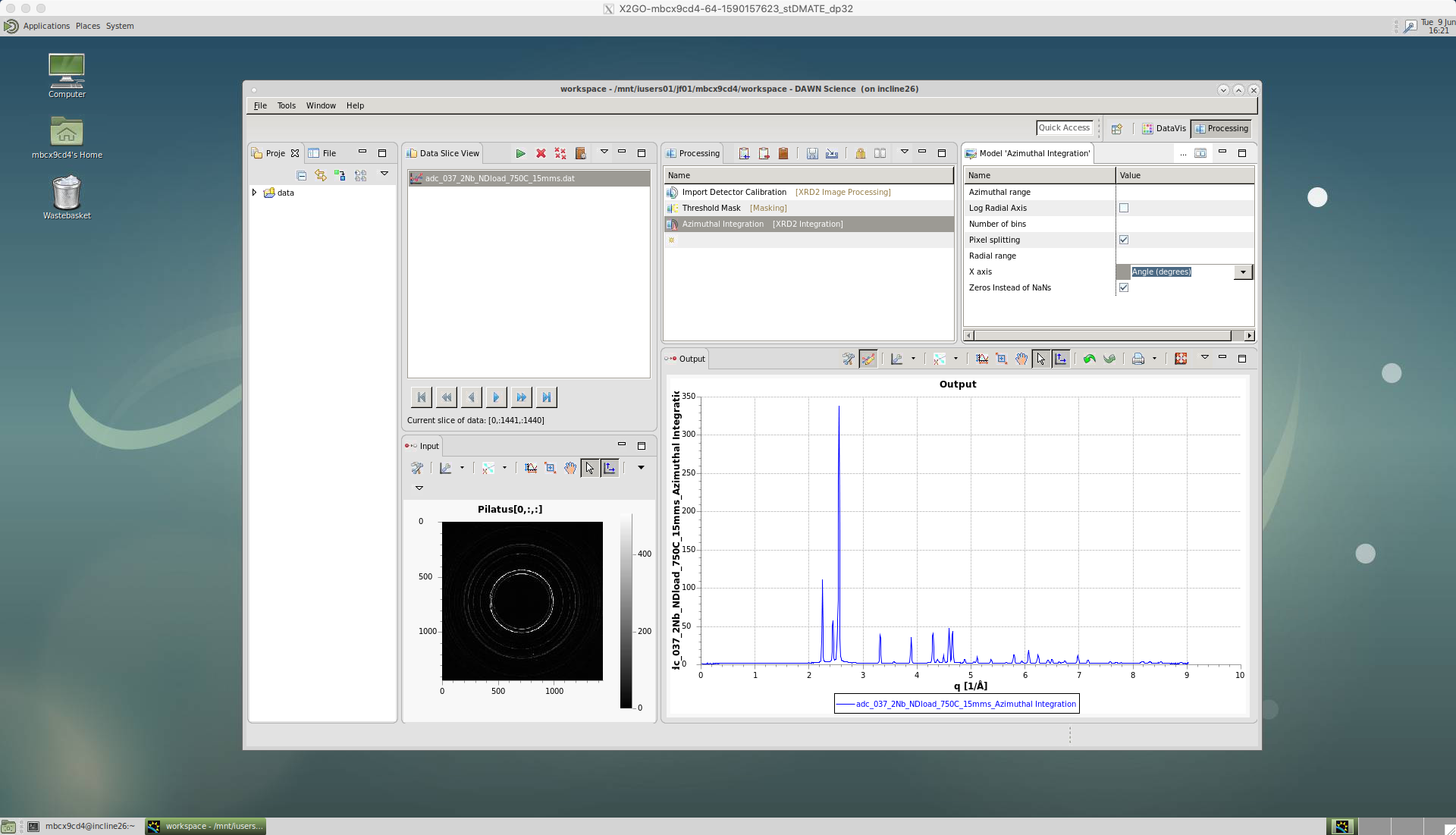
In this case for ‘Export to Text File’ we choose ‘xy’ file format in ‘File Extension’, so that the data can be loaded into TOPAS.
Tick the ‘In separate folder’ box to group the data into one folder.
Leave ‘Pad with zeros’ as five, which should give a high enough number count.
Then, select the ‘Output Directory’, where the data will be saved.
Calibration
[TODO - insert method for calibration]
