Caking SXRD diffraction pattern images using Dioptas and PyFAI

Caking diffraction pattern images using Dioptas and pyFAI on the iCSF

iCSF

You will first need to contact IT services to get setup with an iCSF account. The iCSF (interactive Computational Shared Facility) gives us access to the University’s high performance computing environment. This allows us to store and analyse our large Synchrotron X-ray Diffraction (SXRD) datasets as a group.

What is caking?

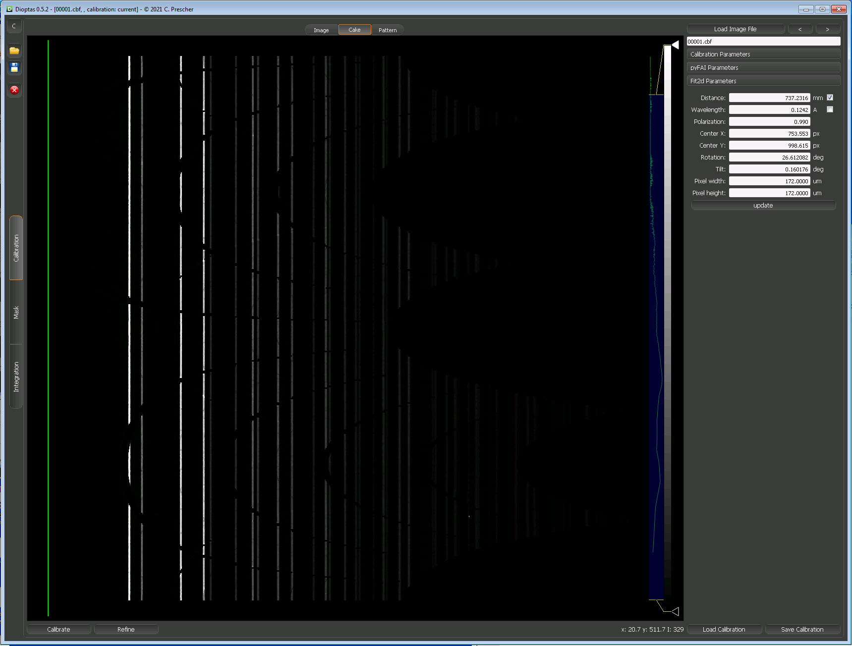
Before we can analyse the diffraction pattern rings for changes in phase fraction, micromechanical response and texture, we need to cake the data. Caking converts our 2-dimensional image into slices (of particular azimuthal angles) to produce a number of intensity profiles versus 2-theta angle (or pixel position). We can then investigate how the intensity peak profile of particular lattice plane peaks change in particular directions over time. We can also run a full azimuthal integration, which sums up the intensities around the whole image, to produce a single intensity profile versus 2-theta angle. This can then be used to calculate the phase fraction, for instance.

Opening Dioptas on the iCSF

To run the caking and azimuthal integration we have setup the program Dioptas on the iCSF. Dioptas is a python-based data analysis and processing program used for processing synchrotron data. The program was developed at the DESY beamline in Germany. It can do the same job as DAWN, but is slightly easier to use and once the calibration files are setup the caking and azimuthal integration can be automated using a python script and the PyFAI package.

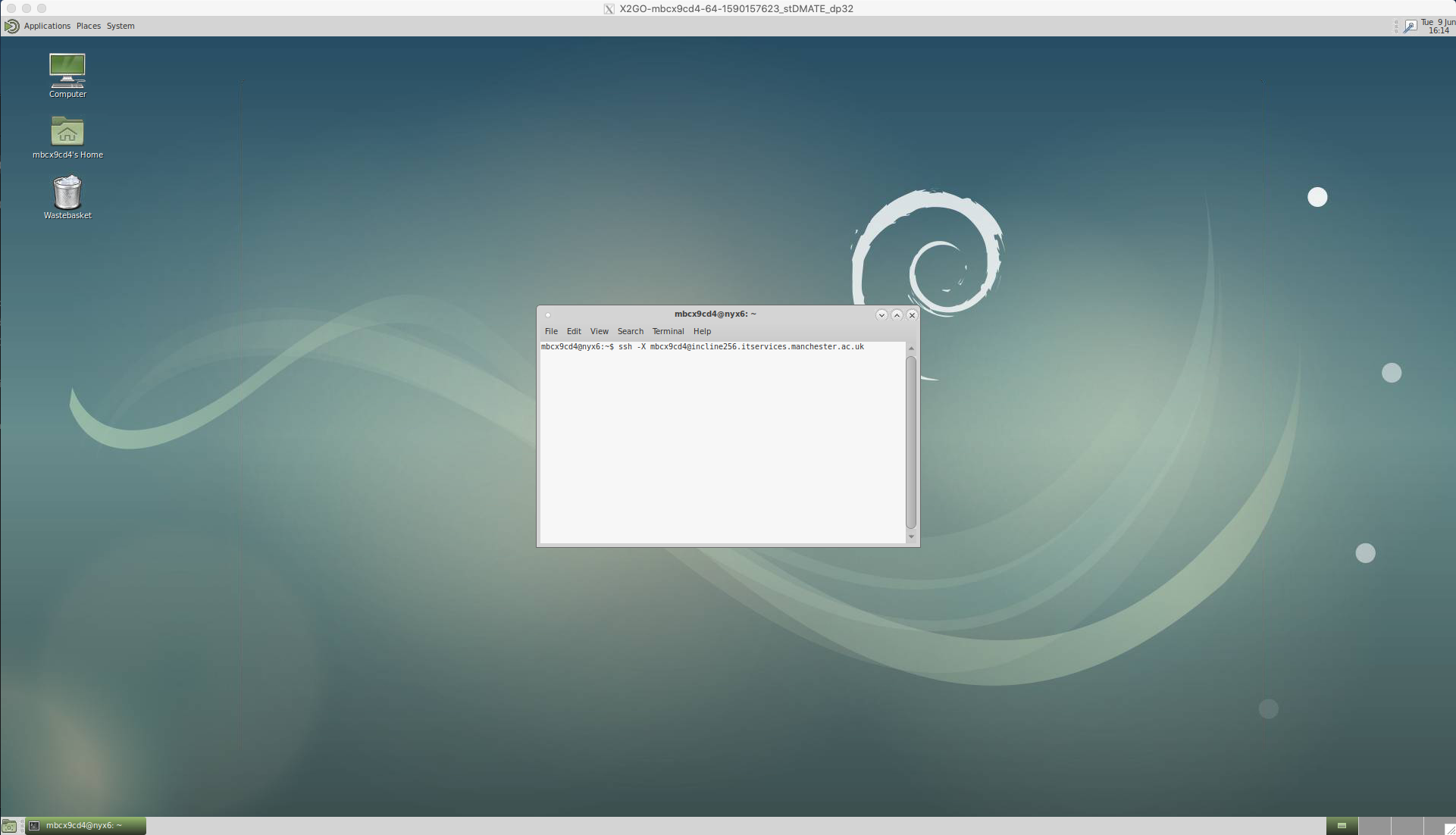
Log onto the iCSF by opening the terminal and using the secure shell (ssh) protocol;

ssh -X mbcx9cd4@incline256.itservices.manchester.ac.uk

You will then be prompted to enter your password.

Load the Dioptas module using the following commands in the terminal;

[TODO]

Creating a .poni calibration file in Dioptas

The documentation for using Dioptas can be found here. However, the following instructions should be enough for a simple calibration.

Start Values

This will then open the Dioptas graphical user interface (GUI).

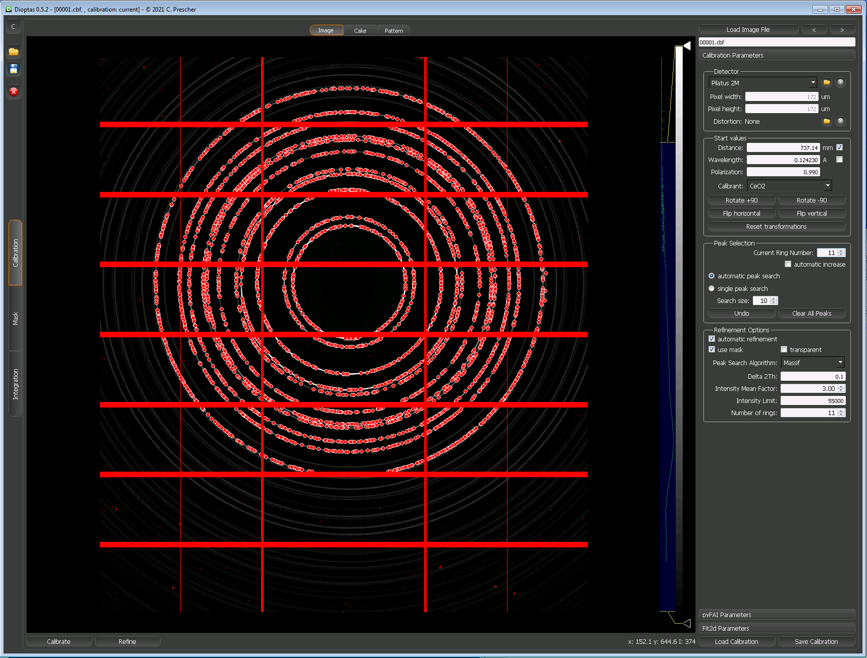
Then, click on ‘Load File’ and select a calibration diffraction pattern.

Select a ‘Custom’ detector and set pixel width and height (e.g. 172 um x 172 um)

Input the distance (e.g. 750 mm) and leave the box ticked as we want to refine this value.

Input the wavelength (e.g. 0.12423 A) and leave the box unticked as we don’t want to refine this value.

Leave polarization as is (0.990).

Select calibrant (e.g. CeO2).

Peak Selection

Untick automatic increase.

Select automatic peak search.

Click ‘clear all peaks’.

Select current ring number as 1.

Then click on the map to select the ring closest to the centre, which will become highlighted with points. You will need to click more than once to select around the entire ring.

Once a ring is fully selected, select the next ring number (2), then click around the next ring away from the centre.

Repeat until 10 or so rings have been selected.

Refinement Options

Make sure automatic refinement is ticked.

Leave the default values in this window, but be sure to change the number of rings to match the number of rings that have been highlighted.

Masking

There is also an option to use a mask, which can filter out any dead pixels or gride lines from the pixel array.

On the far left panel, click on the Mask tab.

In the ‘below thresh’ box type 1 and click on the ‘below thresh’ box. This will highlight all points below a certain threshold.

Note, there is an option to apply a transparent threshold, as well as the standard fill threshold.

Run Calibration

Click ‘Calibrate’ to run a calibration.

Save calibration as .poni file

Click the ‘save calibration’ button at the bottom right of the window and save the calibration as a .poni file.

These two images show the setup just before and just after running a calibration in Dioptas;

Caking and Azimuthal Integration using PyFAI

Dioptas uses elements of FabIO and PyFAI to read in the diffraction images and to perform parts of the calibration. Dioptas also uses PyFAI to perform image integration. However, it is easy to setup a python script using PyFAI to perform the caking or a full azimuthal integration on a set of diffraction image data. A notebook explaining how to do this and the features of PyFAI is available on this link. Some interesting videos explaining how PyFAI works are available on this link.

Load Calibration

First, we load the .poni calibration file, which contains information about the beamline setup. We load an azimuthal integrator object or ai, which we will use to perform an azimuthal integration or caking to the rest of our as-yet ‘uncalibrated’ data.

ai = pyFAI.load("calibration/DLS_CeO2_1200mm.poni")

Azimuthal Integration

An azimuthal integration can be performed using the integrate1d function.

The number of points in 2-theta is defined by the user.
The azimuthal range runs from -180 to 180, or -pi to pi, rather than 0 to 360 as in DAWN.
An output .dat file can be saved, which contains a header of metadata.
The result is returned as a numpy array of 2-theta and intensity.

An azimuthal integration can be performed like this.

result = ai.integrate1d(pattern_image_array,
                        npt=10000,
                        azimuth_range=(-180,180),
                        unit="2th_deg",
                        correctSolidAngle=True,
                        polarization_factor=0.99,
                        method='full_csr',
                        filename="analysis/integrated.dat")

Caking

The integrate2d function is designed for caking of the data. The input arguments are similar to above, but now a number of azimuthal cakes can be chosen.

The following script uses a loop to iterate through some images, create an array for the data and then save it as a text file.

# supress warnings when TIFFs are read
logging.getLogger("fabio.TiffIO").setLevel(logging.ERROR)

# user inputs
number_of_points = 10000
number_of_cakes = 36

# rotate the detector so that the cardinal direction is in the center of the first cake.
first_cake_angle = 360 / number_of_cakes
ai.rot3 = (first_cake_angle / 2) * (math.pi / 180) # convert rotation to radians

# get a list of the files
image_list = sorted(pathlib.Path("data/").glob("pixium*"))

for image_path in image_list:
    # create empty array
    caked_data = np.zeros((number_of_cakes + 1, number_of_points))
    
    # create an image array and cake the data
    with warnings.catch_warnings():
        warnings.simplefilter("ignore")
        image = fabio.open(image_path)
    pattern_image_array = image.data
    result2d = ai.integrate2d(pattern_image_array,
                            number_of_points,
                            number_of_cakes,
                            unit="2th_deg",
                            polarization_factor=0.99,
                            method='full_csr')
    
    # flip the intensity data to order cakes clockwise rather than anticlockwise
    intensity = np.flip(result2d.intensity.T, axis=1)
    
    # reshape radial labels to 2D array so they can be attached to the intensity data.
    radial = np.reshape(result2d.radial, (-1, 1))
    
    result_array = np.hstack((radial, intensity))
    
    # write out the caked data to a text file
    output_path = f"analysis/{image_path.stem}.dat"
    np.savetxt(output_path, result_array)

This caked dataset is now saved in a format that can be used in xrdfit to analyse how the single peak profiles change over time.