Titanium CP/PF modelling - 2021 July

See the project overview for an outline. This page was last updated: July 2021

Next month’s update (August) 🡺

Our initial work focussed on building a dual-phase titanium representative volume element that could be deformed in both “hard” and “soft” loading directions using a crystal plasticity package, DAMASK¹. We will later use the results from these types of simulations to build a new phase map over a subset of the deformed RVE, which can then be fed into a phase-field simulation code to examine, for example, grain growth.

Methodology

RVE construction

We constructed a representative volume element (RVE) of dual-phase titanium composed of a small $\alpha$-phase colony within a $\beta$-phase matrix. Morphologically, the $\alpha$ colony was comprised of three stretched ellipsoids (axis ratio of 2:1:0.4) of the same size positioned semi-randomly (but fixed for all simulations unless otherwise noted) within the $\beta$ matrix, such that individual $\alpha$ laths do not overlap. All $\alpha$ laths were modelled to have the same crystal orientation. The specific orientations of the $\alpha$ and $\beta$ phases were chosen according to the following considerations:

1. The Burgers orientation relationship² specifies an empirically known relationship between the orientations of the HCP $\alpha$ lattice and the BCC $\beta$ lattice, and can be expressed in Miller indices as:

   \[\begin{equation} \begin{split} \{ 0001 \}_\alpha & \parallel \{ 110 \}_\beta \\ \langle 11\bar{2}0\rangle_\alpha & \parallel \langle 111 \rangle_\beta \end{split} \end{equation}\]

2. The planes of the ellipsoidal $\alpha$ laths in dual-phase $\alpha$/$\beta$ titanium are experimentally observed to preferentially lie on a habit plane given by³:

   \[\begin{equation} ( \bar{1}100 )_\alpha\quad\text{or}\quad( \bar{1}12)_\beta \end{equation}\]

3. For convenience, it is desirable for the flat plane of the ellipsoidal $\alpha$ laths to be parallel to one of the model Cartesian planes. This simplifies RVE construction, and reduces the cognitive load when interpreting results. We chose to align the long axes of the ellipsoids with the model $x$-direction.

Given these constraints, we started by identifying a rotation of the hexagonal unit cell such that a “reference” hexagonal unit cell that is aligned with its $a$ and $c$ axes along the model $x$ and $z$ axes, respectively, (which is the alignment system used by DAMASK) is rotated to the frame in which the $( \bar{1}100 )_\alpha$ plane lies within the model $xy$ plane. From inspection, we note that such a rotation can be expressed as the following (pre-multiplying) matrix:

\[\begin{pmatrix} 0 & 0 & 1 \\ \sin{30\degree} & \cos{30\degree} & 0 \\ -\cos{30\degree} & \sin{30\degree} & 0 \end{pmatrix}\text{.}\]

The action of this rotation matrix on the column vectors that form the edges of the hexagonal unit cell is shown in the figure below (blue is the reference unit cell and red is the rotated unit cell):

We then converted the rotation matrix above into a quaternion by first converting to an axis-angle representation, which is 93.84$\degree$ about the Cartesian axis (0.25056281, 0.93511313, 0.25056281), and in turn converting this to a quaternion, which is: (0.6830127, 0.1830127, 0.6830127, 0.1830127). Formulae for these conversions can be found in Rowenhorst et al.⁴. This quaternion was then the starting orientation for all three $\alpha$ laths in the RVE. To find the orientation of the $\beta$ matrix in which the $\alpha$ colony is embedded, we employed the DefDAP Python package⁵; this quaternion is (0.4103, 0.0964, -0.7325, -0.5347).

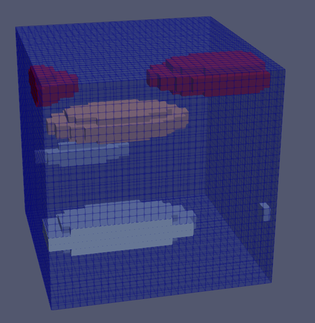
In our initial simulations, we discretised the model geometry into a relatively small number of material points; the grid dimensions were 32 $\times$ 32 $\times$ 32 (32,768 material points). This RVE is shown below. In this way, we benefited from faster throughput in the initial stages of the work. However, we will later use larger grid discretisations, which will be more capable of accurately resolving the stress and strain fields of the deformed RVEs.

The RVE used in our initial simulations of dual-phase Ti. Visualisation using ParaView.

Crystal plasticity model for Ti64

To model plasticity, we employed the phenomenological power law as implemented in DAMASK¹.

Critical resolved shear stresses

We considered two slip systems for the BCC $\beta$ phase and three slip systems for the HCP $\alpha$ phase. The selected critical resolved shear stresses (CRSSs) are listed below. We did not include any hardening.

Phase	Slip plane	Slip direction	Number	CRSS Ref.3) / MPa	CRSS chosen / MPa
$\beta$	$\{110\}$	$\langle 111\rangle$	12	390	390
$\beta$	$\{112\}$	$\langle 111\rangle$	12	-	390
$\alpha$	$\{0001\}$ “basal”	$\langle 11\bar{2}0\rangle$ “a”	3	390	390
$\alpha$	$\{00\bar{1}0\}$ “prismatic”	$\langle 11\bar{2}0\rangle$ “a”	3	390	390
$\alpha$	$\{00\bar{1}1\}$ “pyramidal”	$\langle 11\bar{2}3\rangle$ “c+a”	12	663	663

Loading direction: soft versus hard

We used simple shear along two directions to probe “soft” and “hard” loading directions, with respect to the $\alpha$ phase. Given the chosen CRSS values listed above, a “hard” loading direction would be one that is more closely aligned for activating pyramidal <c+a> slip than basal or prismatic, which are both more easily activated. Considering the aforementioned alignment of the $\alpha$-phase unit cell with respect to our model axes, a “hard” loading direction is thus along the $x$-axis. Conversely, a “soft” loading direction would be along the $y$-axis. Therefore, we performed two simple shear simulations; one along $xz$ (hard) and one along $yz$ (soft). The load cases were specified in terms of deformation gradient rate tensor, $\bold{\dot{F}}$, given below for the hard and soft loading directions, respectively:

\[\begin{align} \bold{\dot{F}}_\textrm{hard} &= \begin{pmatrix} 0 & 0 & 1.0\mathrm{e}{-3}\\ 0 & 0 & 0\\ 0 & 0 & 0 \end{pmatrix} & \bold{\dot{F}}_\textrm{soft} &= \begin{pmatrix} 0 & 0 & 0\\ 0 & 0 & 1.0\mathrm{e}{-3}\\ 0 & 0 & 0 \end{pmatrix} \end{align}\]

The simulations were run for 200 seconds (resulting in an effective total strain of 0.2 in both cases).

Use of MatFlow

We did initial development of the RVE and CP simulation input file generation and simulation output processing using Python script. To improve reproducibility, we will soon integrating the methodology into a MatFlow workflow.

Results

Qualitative analysis: soft versus hard

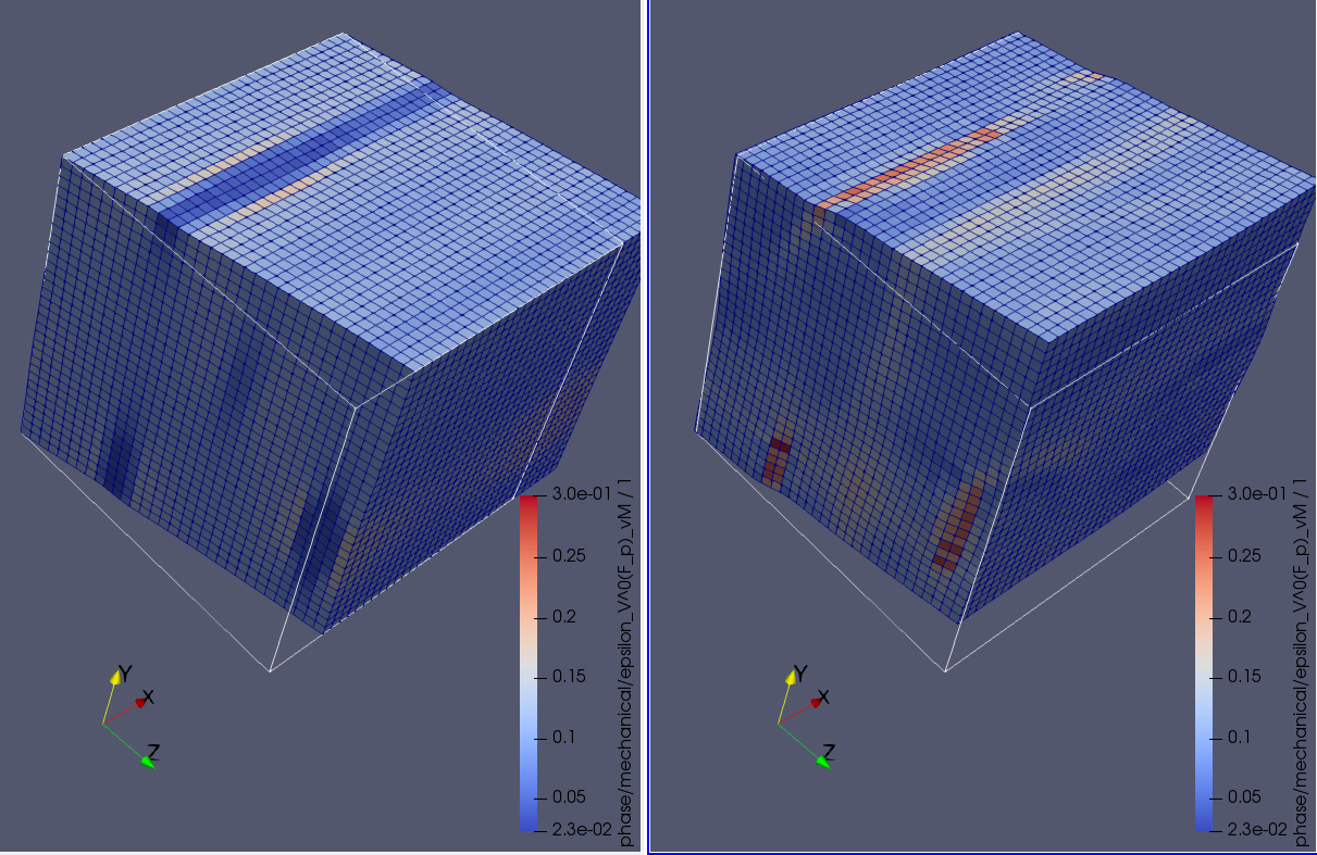
The two simulations were performed using DAMASK v3-alpha3. The results are shown qualitatively in the below figure. For the hard loading direction (on the left), there is very little strain visible in the $\alpha$ laths, relative to the surrounding $\beta$ matrix. On the other hand, for the soft loading direction (on the right), the $\alpha$-laths exhibit much more plastic strain than the $\beta$ matrix.

The deformed RVEs, showing the Von Mises equivalent plastic strain fields; “hard” loading direction on the left and “soft” loading direction on the right. Note that the distinct response of the $\alpha$ laths is visible in both cases. Visualisation using ParaView.

Next steps

1. Investigate methods of generating a new phase map over a region of interest (perhaps a single $\alpha$ lath), according to the formation of deformation-induced sub-grains. This smaller-scale volume element can then be used in a phase-field model to study, for example, grain growth. Two approaches can be pursued: a. Partition the final orientation data (over all voxels) into new “grains” using a clustering algorithm. b. Estimate dislocation density
2. Perform higher-resolution simulations

References and notes