Titanium CP/PF modelling - 2021 October

See the project overview for an outline. This page was last updated: September 2021

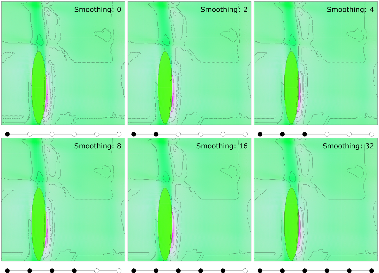
Effect of MTEX FMC smoothing parameter

Effect of MTEX smoothing parameter to smooth grain boundaries of grains clustered using FMC

Getting MTEX-segmentation back into Python

• Our initial approach was to save a PNG image of the grain ID map and load that into Python. Some notes on this approach are listed below:
  • Initially problems with anti-aliasing producing erroneous grain ID map when importing into Python
  • Tried some different methods for saving arrays directly:
    • Matlab’s getframe - not easy to control resolution
    • Saving grains to a .mat file - could not open grains in Python with scipy.io.loadmat and not sure if sufficient information contained in grains.
    • Investigated saving array directly from Matlab figure - figure is comprised of patches and would need to be rasterised/discretised.
  • Eventually found how to switch off anti-aliasing in saving figures
    • set(gcf,'graphicssmoothing','off')
    • results much better now
    • but when rescaling in Python to the size of the simulation slice, some pixels at the edges seem to change grain ID.
    • fix is to turn off interpolation in zoom with the order parameter: grain_IDs_resampled = zoom(grain_IDs, zoom_factor, order=0)
• A better solution was found as follows:
  • Use ebsdsq = gridify(ebsd); to project the (segmented) EBSD map onto a grid (it should already be in an effective grid, but we need to use grid-specific methods)
  • Loop over the coordinates of the EBSD map and use findByLocation to get the grain ID at each grid coordinate
  • Return the grain IDs matrix from the MTEX script and then use the output directly in the invoking MatLab engine invocation.

FMC in MTEX

• Unfortunately, it turns out that MTEX no longer support 3D grain segmentation using FMC. So if we want to perform this analysis in 3D (rather than on 2D slices), we will need to look elsewhere, or implement our own version.

Estimating dislocation density from the crystal plasticity simulation results

We can use the Taylor hardening law to relate the flow stress (or, in our case, the Von Mises “equivalent” stress), $\sigma$ with the dislocation density, $\rho$ ¹:

where $\alpha$ is a material parameter, $G$ is the shear modulus, and $b$ is the Burgers vector.

Voronoi tessellation of seed points according to dislocation density

With a dislocation density field, $\rho$ defined over the model slice, we can generate seed points on the slice that have a commensurate density. To this we can use the “random choice” function within Numpy, which allows selecting N random indices, where each can be assigned a selection probability. In our case, we set this probability to be the dislocation density field:

import numpy as np

rho # dislocation density grid

rho_flat = rho.flatten() # create a flat copy of the array
rho_flat /= rho_flat.sum()  # probabilities array should sum to one

rng = np.random.default_rng()
sample_index = rng.choice(a=rho_flat.size, p=rho_flat, size=(number,))

# Convert back to an array of 2D row vectors, where each row represents integer grid coordinates:
seeds = np.vstack(np.unravel_index(sample_index, rho.shape)).T

To perform the Voronoi tessellation (for the set of seed points that fall within each sub-grain), we then need to consider again the periodicity.

References